Getting Started

Basic Usage

The main interface is the Benchmark class with a context manager API:

from zeropybench import Benchmark

bench = Benchmark()

data = range(1000)
with bench():
    sum(data)

14.547 µs ± 0.18% (median of 7 runs, 20000 loops each)

Multidimensional Benchmarking

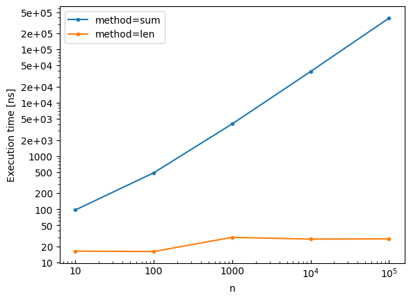
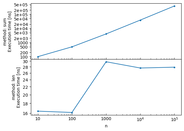
Tag your benchmarks with arbitrary keyword arguments to compare different methods and parameters:

bench = Benchmark()

for n in [10, 100, 1000, 10_000, 100_000]:
    data = list(range(n))
    with bench(method='sum', n=n):
        sum(data)
    with bench(method='len', n=n):
        len(data)

method=sum, n=10: 97.126 ns ± 0.23% (median of 7 runs, 2000000 loops each)
method=len, n=10: 16.383 ns ± 7.00% (median of 7 runs, 20000000 loops each)
method=sum, n=100: 484.399 ns ± 0.32% (median of 7 runs, 500000 loops each)
method=len, n=100: 16.125 ns ± 2.49% (median of 7 runs, 20000000 loops each)
method=sum, n=1000: 4.005 µs ± 0.07% (median of 7 runs, 50000 loops each)
method=len, n=1000: 29.755 ns ± 2.66% (median of 7 runs, 10000000 loops each)
method=sum, n=10000: 38.528 µs ± 0.02% (median of 7 runs, 5000 loops each)
method=len, n=10000: 27.590 ns ± 1.52% (median of 7 runs, 10000000 loops each)
method=sum, n=100000: 387.244 µs ± 0.15% (median of 7 runs, 500 loops each)
method=len, n=100000: 27.869 ns ± 1.45% (median of 7 runs, 10000000 loops each)

Viewing Results

Display the benchmark results as a table:

print(bench)

┌───┬────────┬─────────┬────────────────────────────┬──────────┐
│   ┆ method ┆ n       ┆ median_execution_time (ns) ┆ ± (%)    │
╞═══╪════════╪═════════╪════════════════════════════╪══════════╡
│ 0 ┆ sum    ┆ 10      ┆ 97.125852                  ┆ 0.23407  │
│ 1 ┆ len    ┆ 10      ┆ 16.38264                   ┆ 6.996066 │
│ 2 ┆ sum    ┆ 100     ┆ 484.399138                 ┆ 0.316887 │
│ 3 ┆ len    ┆ 100     ┆ 16.124628                  ┆ 2.494701 │
│ 4 ┆ sum    ┆ 1_000   ┆ 4_005.20688                ┆ 0.073634 │
│ 5 ┆ len    ┆ 1_000   ┆ 29.755391                  ┆ 2.656737 │
│ 6 ┆ sum    ┆ 10_000  ┆ 38_527.9164                ┆ 0.0152   │
│ 7 ┆ len    ┆ 10_000  ┆ 27.590323                  ┆ 1.517248 │
│ 8 ┆ sum    ┆ 100_000 ┆ 387_243.763998             ┆ 0.152063 │
│ 9 ┆ len    ┆ 100_000 ┆ 27.868963                  ┆ 1.445575 │
└───┴────────┴─────────┴────────────────────────────┴──────────┘

Accessing Raw Data

Benchmark runs can be accessed individually:

from pprint import pprint

pprint(bench[4], sort_dicts=False)

{'method': 'sum',
 'n': 1000,
 'median_execution_time': 4.005206879992329e-06,
 'execution_times': [5.015862200016272e-06,
                     4.005206879992329e-06,
                     4.003217680001398e-06,
                     4.0036172799955235e-06,
                     4.0035506799904394e-06,
                     4.169566679993295e-06,
                     4.18522888001462e-06]}

Note

All time measurements in the raw data are in seconds.

To get the benchmark data as a list of dictionaries:

bench.to_dicts()[:4]

[{'method': 'sum',
  'n': 10,
  'median_execution_time': 9.712585150009545e-08,
  'execution_times': [1.0844265300056576e-07,
   9.738626150010531e-08,
   9.651124149968382e-08,
   9.712585150009545e-08,
   9.703353149961913e-08,
   9.697251099987624e-08,
   9.715665099975013e-08]},
 {'method': 'len',
  'n': 10,
  'median_execution_time': 1.6382640400024683e-08,
  'execution_times': [1.8868343200028903e-08,
   1.666911545007679e-08,
   1.5609579349984415e-08,
   1.5372362849939236e-08,
   1.4789448749979783e-08,
   1.6395481400013523e-08,
   1.6382640400024683e-08]},
 {'method': 'sum',
  'n': 100,
  'median_execution_time': 4.84399138000299e-07,
  'execution_times': [5.668098679998366e-07,
   4.833033779977996e-07,
   4.833637960000488e-07,
   4.845398159995966e-07,
   4.84399138000299e-07,
   4.84926778000954e-07,
   4.833189759992819e-07]},
 {'method': 'len',
  'n': 100,
  'median_execution_time': 1.6124628400029905e-08,
  'execution_times': [1.7196918500030732e-08,
   1.5798782349975228e-08,
   1.6124628400029905e-08,
   1.5693608849960583e-08,
   1.621016540002529e-08,
   1.63959499500379e-08,
   1.607470889994147e-08]}]

Or as a Polars DataFrame:

bench.to_dataframe()

shape: (10, 4)

method	n	median_execution_time	execution_times
str	i64	f64	list[f64]
"sum"	10	9.7126e-8	[1.0844e-7, 9.7386e-8, … 9.7157e-8]
"len"	10	1.6383e-8	[1.8868e-8, 1.6669e-8, … 1.6383e-8]
"sum"	100	4.8440e-7	[5.6681e-7, 4.8330e-7, … 4.8332e-7]
"len"	100	1.6125e-8	[1.7197e-8, 1.5799e-8, … 1.6075e-8]
"sum"	1000	0.000004	[0.000005, 0.000004, … 0.000004]
"len"	1000	2.9755e-8	[3.0839e-8, 2.8677e-8, … 2.9755e-8]
"sum"	10000	0.000039	[0.000047, 0.000039, … 0.000039]
"len"	10000	2.7590e-8	[2.9765e-8, 2.7575e-8, … 2.7309e-8]
"sum"	100000	0.000387	[0.000469, 0.000414, … 0.000387]
"len"	100000	2.7869e-8	[3.0573e-8, 2.7583e-8, … 2.8911e-8]

Exporting Benchmark Results

Benchmarks can be saved in various formats such as CSV:

bench.write_csv('results.csv')

Parquet:

bench.write_parquet('results.parquet')

or MarkDown:

bench.write_markdown('results.md')

Importing Benchmarks Results

Benchmarks saved as CSV or Parquet files can be imported:

from zeropybench import read_benchmark

bench = read_benchmark('results.csv')

Plotting Results

Visualize benchmark results with built-in plotting:

bench.plot()

Save the plot to a file:

bench.write_plot('results.pdf')

Subplots

Create subplots using the by parameter:

# Create subplots by method
bench.plot(by='method')

Speedup Plots with Reference

Use the reference parameter to add a speedup subplot comparing all methods to a baseline. The speedup is computed as reference_time / method_time, so values > 1 mean faster than the reference:

# Reload the benchmark data
bench = Benchmark()

for n in [100, 1000, 10000]:
    data = list(range(n))
    with bench(method='sum', n=n):
        sum(data)
    with bench(method='len', n=n):
        len(data)

# Plot with speedup comparison against 'sum'
bench.plot(reference='sum')

method=sum, n=100: 484.071 ns ± 0.14% (median of 7 runs, 500000 loops each)
method=len, n=100: 17.392 ns ± 1.52% (median of 7 runs, 20000000 loops each)
method=sum, n=1000: 4.003 µs ± 0.11% (median of 7 runs, 50000 loops each)
method=len, n=1000: 28.823 ns ± 1.78% (median of 7 runs, 10000000 loops each)
method=sum, n=10000: 43.828 µs ± 0.20% (median of 7 runs, 5000 loops each)
method=len, n=10000: 28.954 ns ± 4.45% (median of 7 runs, 10000000 loops each)

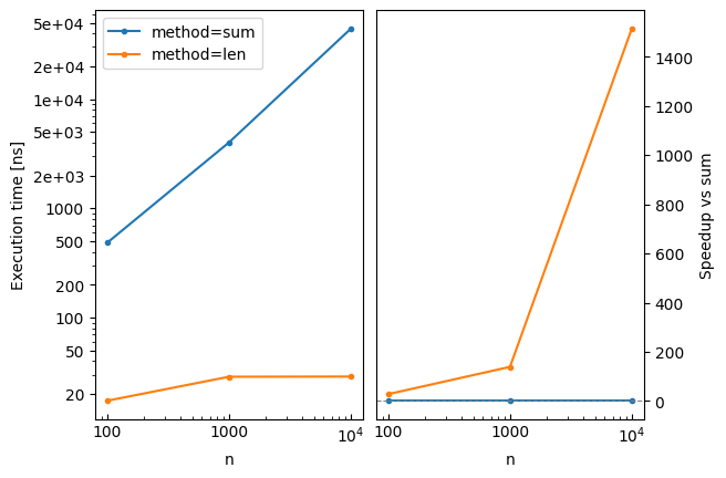
The plot legend can also be used to select the reference with reference='method=sum', which is handy for multi-dimensional benchmarks.

Configuration Options

Customize the benchmark behavior:

bench = Benchmark(
    repeat=10,  # Number of measurement repetitions
    min_duration_per_repeat=0.5,  # Minimum duration per repeat (seconds)
    verbose=True,  # Print the setup and benchmarked code
)

data = list(range(1000))
with bench():
    sum(data)

Benchmarked code:
    sum(data)
4.187 µs ± 0.12% (median of 10 runs, 100000 loops each)

Loading Benchmark Data

Use read_benchmark to load benchmark results from a CSV or Parquet file:

from zeropybench import read_benchmark

# Load benchmark results from CSV
bench = read_benchmark('results.csv')

# Or from Parquet
bench = read_benchmark('results.parquet')

# Display results
print(bench)

# Create plots
bench.plot(x='n', by='method')

The file should have been created with bench.write_csv() or bench.write_parquet(). The metadata (repeat, min_duration_per_repeat) are automatically restored from the file.