Getting Started

Basic Usage

The main interface is the Benchmark class with a context manager API:

from zeropybench import Benchmark

bench = Benchmark()

data = range(1000)
with bench():
    sum(data)

16.402 µs ± 0.32% (median of 7 runs, 20000 loops each)

Multidimensional Benchmarking

Tag your benchmarks with arbitrary keyword arguments to compare different methods and parameters:

bench = Benchmark()

for n in [10, 100, 1000, 10_000, 100_000]:
    data = list(range(n))
    with bench(method='sum', n=n):
        sum(data)
    with bench(method='len', n=n):
        len(data)

method=sum, n=10: 102.325 ns ± 1.09% (median of 7 runs, 2000000 loops each)
method=len, n=10: 16.126 ns ± 2.45% (median of 7 runs, 20000000 loops each)
method=sum, n=100: 515.954 ns ± 0.42% (median of 7 runs, 500000 loops each)
method=len, n=100: 16.106 ns ± 1.43% (median of 7 runs, 20000000 loops each)
method=sum, n=1000: 4.412 µs ± 2.05% (median of 7 runs, 50000 loops each)
method=len, n=1000: 33.687 ns ± 0.56% (median of 7 runs, 10000000 loops each)
method=sum, n=10000: 43.728 µs ± 1.34% (median of 7 runs, 5000 loops each)
method=len, n=10000: 34.292 ns ± 1.68% (median of 7 runs, 10000000 loops each)
method=sum, n=100000: 441.424 µs ± 2.35% (median of 7 runs, 500 loops each)
method=len, n=100000: 33.915 ns ± 1.04% (median of 7 runs, 10000000 loops each)

Viewing Results

Display the benchmark results as a table:

print(bench)

┌───┬────────┬─────────┬────────────────────────────┬──────────┐
│   ┆ method ┆ n       ┆ median_execution_time (ns) ┆ ± (%)    │
╞═══╪════════╪═════════╪════════════════════════════╪══════════╡
│ 0 ┆ sum    ┆ 10      ┆ 102.325327                 ┆ 1.090091 │
│ 1 ┆ len    ┆ 10      ┆ 16.126158                  ┆ 2.448888 │
│ 2 ┆ sum    ┆ 100     ┆ 515.953836                 ┆ 0.424632 │
│ 3 ┆ len    ┆ 100     ┆ 16.106147                  ┆ 1.432613 │
│ 4 ┆ sum    ┆ 1_000   ┆ 4_412.19106                ┆ 2.050203 │
│ 5 ┆ len    ┆ 1_000   ┆ 33.686808                  ┆ 0.556321 │
│ 6 ┆ sum    ┆ 10_000  ┆ 43_728.288                 ┆ 1.336406 │
│ 7 ┆ len    ┆ 10_000  ┆ 34.291856                  ┆ 1.678234 │
│ 8 ┆ sum    ┆ 100_000 ┆ 441_424.463999             ┆ 2.349386 │
│ 9 ┆ len    ┆ 100_000 ┆ 33.914807                  ┆ 1.035496 │
└───┴────────┴─────────┴────────────────────────────┴──────────┘

Accessing Raw Data

Benchmark runs can be accessed individually:

from pprint import pprint

pprint(bench[4], sort_dicts=False)

{'method': 'sum',
 'n': 1000,
 'median_execution_time': 4.4121910600006235e-06,
 'execution_times': [4.469164060028561e-06,
                     4.34961718001432e-06,
                     4.5160771000155365e-06,
                     4.4121910600006235e-06,
                     4.380171119992156e-06,
                     4.577699759975075e-06,
                     4.351177399985318e-06]}

Note

All time measurements in the raw data are in seconds.

To get the benchmark data as a list of dictionaries:

bench.to_dicts()[:4]

[{'method': 'sum',
  'n': 10,
  'median_execution_time': 1.0232532700047159e-07,
  'execution_times': [1.0318430650022492e-07,
   1.0157297349996952e-07,
   1.0161972449986933e-07,
   1.0391915499985771e-07,
   1.0232532700047159e-07,
   1.0523975300020538e-07,
   1.0214908899979491e-07]},
 {'method': 'len',
  'n': 10,
  'median_execution_time': 1.612615840003855e-08,
  'execution_times': [1.7377404299986665e-08,
   1.7177271350010414e-08,
   1.5961622050053847e-08,
   1.6076252550010394e-08,
   1.63925226000174e-08,
   1.612615840003855e-08,
   1.5824635650005802e-08]},
 {'method': 'sum',
  'n': 100,
  'median_execution_time': 5.159538359985163e-07,
  'execution_times': [5.159538359985163e-07,
   5.24601545999758e-07,
   5.135483339981875e-07,
   5.156132299998717e-07,
   5.172660980024375e-07,
   5.144760920011322e-07,
   5.208825640002033e-07]},
 {'method': 'len',
  'n': 100,
  'median_execution_time': 1.6106147049958962e-08,
  'execution_times': [1.9216336550016423e-08,
   1.8061450799996238e-08,
   1.601641600000221e-08,
   1.5950515849999646e-08,
   1.5928987950064767e-08,
   1.6165243099931105e-08,
   1.6106147049958962e-08]}]

Or as a Polars DataFrame:

bench.to_dataframe()

shape: (10, 4)

method	n	median_execution_time	execution_times
str	i64	f64	list[f64]
"sum"	10	1.0233e-7	[1.0318e-7, 1.0157e-7, … 1.0215e-7]
"len"	10	1.6126e-8	[1.7377e-8, 1.7177e-8, … 1.5825e-8]
"sum"	100	5.1595e-7	[5.1595e-7, 5.2460e-7, … 5.2088e-7]
"len"	100	1.6106e-8	[1.9216e-8, 1.8061e-8, … 1.6106e-8]
"sum"	1000	0.000004	[0.000004, 0.000004, … 0.000004]
"len"	1000	3.3687e-8	[3.5459e-8, 3.3555e-8, … 3.3582e-8]
"sum"	10000	0.000044	[0.000043, 0.000043, … 0.000044]
"len"	10000	3.4292e-8	[3.4738e-8, 3.4292e-8, … 3.3671e-8]
"sum"	100000	0.000441	[0.000441, 0.000457, … 0.000451]
"len"	100000	3.3915e-8	[3.4480e-8, 3.4286e-8, … 3.3915e-8]

Exporting Benchmark Results

Benchmarks can be saved in various formats such as CSV:

bench.write_csv('results.csv')

Parquet:

bench.write_parquet('results.parquet')

or MarkDown:

bench.write_markdown('results.md')

Importing Benchmarks Results

Benchmarks saved as CSV or Parquet files can be imported:

from zeropybench import read_benchmark

bench = read_benchmark('results.csv')

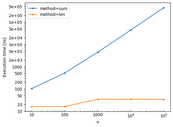
Plotting Results

Visualize benchmark results with built-in plotting:

bench.plot()

Save the plot to a file:

bench.write_plot('results.pdf')

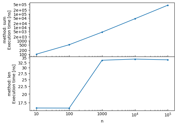
Subplots

Create subplots using the by parameter:

# Create subplots by method
bench.plot(by='method')

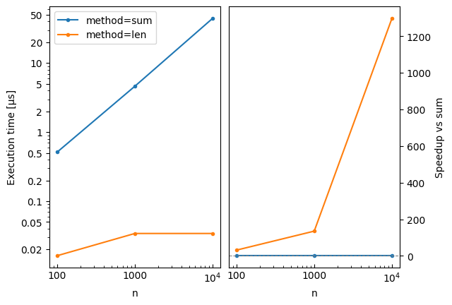
Speedup Plots with Reference

Use the reference parameter to add a speedup subplot comparing all methods to a baseline. The speedup is computed as reference_time / method_time, so values > 1 mean faster than the reference:

# Reload the benchmark data
bench = Benchmark()

for n in [100, 1000, 10000]:
    data = list(range(n))
    with bench(method='sum', n=n):
        sum(data)
    with bench(method='len', n=n):
        len(data)

# Plot with speedup comparison against 'sum'
bench.plot(reference='sum')

method=sum, n=100: 513.510 ns ± 1.26% (median of 7 runs, 500000 loops each)
method=len, n=100: 16.250 ns ± 1.67% (median of 7 runs, 20000000 loops each)
method=sum, n=1000: 4.616 µs ± 2.54% (median of 7 runs, 50000 loops each)
method=len, n=1000: 34.104 ns ± 0.43% (median of 7 runs, 10000000 loops each)
method=sum, n=10000: 44.255 µs ± 0.55% (median of 7 runs, 5000 loops each)
method=len, n=10000: 34.112 ns ± 1.02% (median of 7 runs, 10000000 loops each)

The plot legend can also be used to select the reference with reference='method=sum', which is handy for multi-dimensional benchmarks.

Configuration Options

Customize the benchmark behavior:

bench = Benchmark(
    repeat=10,  # Number of measurement repetitions
    min_duration_per_repeat=0.5,  # Minimum duration per repeat (seconds)
    verbose=True,  # Print the setup and benchmarked code
)

data = list(range(1000))
with bench():
    sum(data)

Benchmarked code:
    sum(data)
4.630 µs ± 0.42% (median of 10 runs, 200000 loops each)

Loading Benchmark Data

Use read_benchmark to load benchmark results from a CSV or Parquet file:

from zeropybench import read_benchmark

# Load benchmark results from CSV
bench = read_benchmark('results.csv')

# Or from Parquet
bench = read_benchmark('results.parquet')

# Display results
print(bench)

# Create plots
bench.plot(x='n', by='method')

The file should have been created with bench.write_csv() or bench.write_parquet(). The metadata (repeat, min_duration_per_repeat) are automatically restored from the file.