JAX Examples
Basic JAX Benchmarking
ZeroPyBench automatically detects JAX arrays in your code and wraps the benchmarked expression in a JIT-compiled function.
Note
For JAX benchmarking, ZeroPyBench provides additional measurements, see below.
import jax
import jax.numpy as jnp
import jax.random as jr

from zeropybench import Benchmark

bench = Benchmark(repeat=20)
x = jnp.ones(1000)
y = jnp.ones(1000)

with bench():
    x + y
10.933 µs ± 1.53% (median of 20 runs, 20000 loops each)
Verbose Mode
Use verbose=True to see the setup code (JIT-compiled function) and the benchmarked code:
bench = Benchmark(verbose=True)

with bench():
    x + y
Setup code:
    @jax.jit
    def __bench_func(x, y):
        return x + y
Benchmarked code:
    __bench_func(x, y).block_until_ready()
10.911 µs ± 1.50% (median of 7 runs, 20000 loops each)
For functions returning a PyTree (e.g., a tuple of Arrays), the slightly slower jax.block_until_ready is used instead.
from dataclasses import dataclass


@jax.tree_util.register_dataclass
@dataclass
class Vector:
    x: jax.Array
    y: jax.Array

    @classmethod
    def normal(cls, key, shape):
        key_x, key_y = jr.split(key)
        return Vector(jr.normal(key_x, shape), jr.normal(key_y, shape))

    def __add__(self, other):
        if not isinstance(other, Vector):
            return NotImplemented
        return Vector(self.x + other.x, self.y + other.y)


key1, key2 = jr.split(jr.key(42))
shape = (100,)
v1 = Vector.normal(key1, shape)
v2 = Vector.normal(key2, shape)

bench = Benchmark(verbose=True)
with bench():
    v1 + v2
Setup code:
    @jax.jit
    def __bench_func(v1, v2):
        return v1 + v2
Benchmarked code:
    jax.block_until_ready(__bench_func(v1, v2))
17.362 µs ± 0.54% (median of 7 runs, 20000 loops each)
Multiple Bare Expressions
When the benchmarked code contains several bare expressions (without assignment), they are each captured into temporary variables so that block_until_ready can synchronize all computations. Calls to functions known to return None (such as print or functions annotated with -> None) are left as-is:
bench = Benchmark(verbose=True)

with bench():
    print(x)
    x + y
    x * y
[1. 1. 1. 1. 1. 1. 1. 1. 1. 1. 1. 1. 1. 1. 1. 1. 1. 1. 1. 1. 1. 1. 1. 1.
 1. 1. 1. 1. 1. 1. 1. 1. 1. 1. 1. 1. 1. 1. 1. 1. 1. 1. 1. 1. 1. 1. 1. 1.
 1. 1. 1. 1. 1. 1. 1. 1. 1. 1. 1. 1. 1. 1. 1. 1. 1. 1. 1. 1. 1. 1. 1. 1.
 1. 1. 1. 1. 1. 1. 1. 1. 1. 1. 1. 1. 1. 1. 1. 1. 1. 1. 1. 1. 1. 1. 1. 1.
 1. 1. 1. 1. 1. 1. 1. 1. 1. 1. 1. 1. 1. 1. 1. 1. 1. 1. 1. 1. 1. 1. 1. 1.
 1. 1. 1. 1. 1. 1. 1. 1. 1. 1. 1. 1. 1. 1. 1. 1. 1. 1. 1. 1. 1. 1. 1. 1.
 1. 1. 1. 1. 1. 1. 1. 1. 1. 1. 1. 1. 1. 1. 1. 1. 1. 1. 1. 1. 1. 1. 1. 1.
 1. 1. 1. 1. 1. 1. 1. 1. 1. 1. 1. 1. 1. 1. 1. 1. 1. 1. 1. 1. 1. 1. 1. 1.
 1. 1. 1. 1. 1. 1. 1. 1. 1. 1. 1. 1. 1. 1. 1. 1. 1. 1. 1. 1. 1. 1. 1. 1.
 1. 1. 1. 1. 1. 1. 1. 1. 1. 1. 1. 1. 1. 1. 1. 1. 1. 1. 1. 1. 1. 1. 1. 1.
 1. 1. 1. 1. 1. 1. 1. 1. 1. 1. 1. 1. 1. 1. 1. 1. 1. 1. 1. 1. 1. 1. 1. 1.
 1. 1. 1. 1. 1. 1. 1. 1. 1. 1. 1. 1. 1. 1. 1. 1. 1. 1. 1. 1. 1. 1. 1. 1.
 1. 1. 1. 1. 1. 1. 1. 1. 1. 1. 1. 1. 1. 1. 1. 1. 1. 1. 1. 1. 1. 1. 1. 1.
 1. 1. 1. 1. 1. 1. 1. 1. 1. 1. 1. 1. 1. 1. 1. 1. 1. 1. 1. 1. 1. 1. 1. 1.
 1. 1. 1. 1. 1. 1. 1. 1. 1. 1. 1. 1. 1. 1. 1. 1. 1. 1. 1. 1. 1. 1. 1. 1.
 1. 1. 1. 1. 1. 1. 1. 1. 1. 1. 1. 1. 1. 1. 1. 1. 1. 1. 1. 1. 1. 1. 1. 1.
 1. 1. 1. 1. 1. 1. 1. 1. 1. 1. 1. 1. 1. 1. 1. 1. 1. 1. 1. 1. 1. 1. 1. 1.
 1. 1. 1. 1. 1. 1. 1. 1. 1. 1. 1. 1. 1. 1. 1. 1. 1. 1. 1. 1. 1. 1. 1. 1.
 1. 1. 1. 1. 1. 1. 1. 1. 1. 1. 1. 1. 1. 1. 1. 1. 1. 1. 1. 1. 1. 1. 1. 1.
 1. 1. 1. 1. 1. 1. 1. 1. 1. 1. 1. 1. 1. 1. 1. 1. 1. 1. 1. 1. 1. 1. 1. 1.
 1. 1. 1. 1. 1. 1. 1. 1. 1. 1. 1. 1. 1. 1. 1. 1. 1. 1. 1. 1. 1. 1. 1. 1.
 1. 1. 1. 1. 1. 1. 1. 1. 1. 1. 1. 1. 1. 1. 1. 1. 1. 1. 1. 1. 1. 1. 1. 1.
 1. 1. 1. 1. 1. 1. 1. 1. 1. 1. 1. 1. 1. 1. 1. 1. 1. 1. 1. 1. 1. 1. 1. 1.
 1. 1. 1. 1. 1. 1. 1. 1. 1. 1. 1. 1. 1. 1. 1. 1. 1. 1. 1. 1. 1. 1. 1. 1.
 1. 1. 1. 1. 1. 1. 1. 1. 1. 1. 1. 1. 1. 1. 1. 1. 1. 1. 1. 1. 1. 1. 1. 1.
 1. 1. 1. 1. 1. 1. 1. 1. 1. 1. 1. 1. 1. 1. 1. 1. 1. 1. 1. 1. 1. 1. 1. 1.
 1. 1. 1. 1. 1. 1. 1. 1. 1. 1. 1. 1. 1. 1. 1. 1. 1. 1. 1. 1. 1. 1. 1. 1.
 1. 1. 1. 1. 1. 1. 1. 1. 1. 1. 1. 1. 1. 1. 1. 1. 1. 1. 1. 1. 1. 1. 1. 1.
 1. 1. 1. 1. 1. 1. 1. 1. 1. 1. 1. 1. 1. 1. 1. 1. 1. 1. 1. 1. 1. 1. 1. 1.
 1. 1. 1. 1. 1. 1. 1. 1. 1. 1. 1. 1. 1. 1. 1. 1. 1. 1. 1. 1. 1. 1. 1. 1.
 1. 1. 1. 1. 1. 1. 1. 1. 1. 1. 1. 1. 1. 1. 1. 1. 1. 1. 1. 1. 1. 1. 1. 1.
 1. 1. 1. 1. 1. 1. 1. 1. 1. 1. 1. 1. 1. 1. 1. 1. 1. 1. 1. 1. 1. 1. 1. 1.
 1. 1. 1. 1. 1. 1. 1. 1. 1. 1. 1. 1. 1. 1. 1. 1. 1. 1. 1. 1. 1. 1. 1. 1.
 1. 1. 1. 1. 1. 1. 1. 1. 1. 1. 1. 1. 1. 1. 1. 1. 1. 1. 1. 1. 1. 1. 1. 1.
 1. 1. 1. 1. 1. 1. 1. 1. 1. 1. 1. 1. 1. 1. 1. 1. 1. 1. 1. 1. 1. 1. 1. 1.
 1. 1. 1. 1. 1. 1. 1. 1. 1. 1. 1. 1. 1. 1. 1. 1. 1. 1. 1. 1. 1. 1. 1. 1.
 1. 1. 1. 1. 1. 1. 1. 1. 1. 1. 1. 1. 1. 1. 1. 1. 1. 1. 1. 1. 1. 1. 1. 1.
 1. 1. 1. 1. 1. 1. 1. 1. 1. 1. 1. 1. 1. 1. 1. 1. 1. 1. 1. 1. 1. 1. 1. 1.
 1. 1. 1. 1. 1. 1. 1. 1. 1. 1. 1. 1. 1. 1. 1. 1. 1. 1. 1. 1. 1. 1. 1. 1.
 1. 1. 1. 1. 1. 1. 1. 1. 1. 1. 1. 1. 1. 1. 1. 1. 1. 1. 1. 1. 1. 1. 1. 1.
 1. 1. 1. 1. 1. 1. 1. 1. 1. 1. 1. 1. 1. 1. 1. 1. 1. 1. 1. 1. 1. 1. 1. 1.
 1. 1. 1. 1. 1. 1. 1. 1. 1. 1. 1. 1. 1. 1. 1. 1.]
JitTracer(float32[1000])
Setup code:
    @jax.jit
    def __bench_func(x, y):
        print(x)
        __expr1 = x + y
        __expr2 = x * y
        return (__expr1, __expr2)
Benchmarked code:
    jax.block_until_ready(__bench_func(x, y))
18.335 µs ± 0.30% (median of 7 runs, 20000 loops each)
JAX-Specific Report Fields
When JAX code is detected, the benchmark report includes additional fields
first_execution_time: The execution time of the code inside the context manager, which usually correspond to the non-jitted version of the code that is being benchmarked.compilation_time: the lowering and compilation time.generated_code_size: the total size of the generated machine code in bytes, including embedded constants.temp_size: the size of the preallocated temporary buffer arena in bytes. This accounts for intermediate buffers needed during execution, excluding input arguments, outputs, and constants.
Warning
The generated_code_size and temp_size values may not be reliable on the CPU backend.
print(bench)
run = bench[0]
print('Execution times [μs]:', sorted(_ * 1e6 for _ in run['execution_times']))
┌───┬─────────────────┬─────────┬────────────────┬────────────────┬────────────────┬───────────────┐
│   ┆ median_executio ┆ ± (%)   ┆ first_executio ┆ compilation_ti ┆ generated_code ┆ temp_size (B) │
│   ┆ n_time (µs)     ┆         ┆ n_time (µs)    ┆ me (µs)        ┆ _size (B)      ┆               │
╞═══╪═════════════════╪═════════╪════════════════╪════════════════╪════════════════╪═══════════════╡
│ 0 ┆ 18.33455        ┆ 0.30375 ┆ 69_099.015     ┆ 42_941.605001  ┆ 0              ┆ 0             │
└───┴─────────────────┴─────────┴────────────────┴────────────────┴────────────────┴───────────────┘
Execution times [μs]: [18.296987099984108, 18.29739115000848, 18.30585774996507, 18.334550300005503, 18.375897999976587, 18.5337957500451, 18.59731534996172]
Visualizing the HLO
The hlo field contains the StableHLO representation of the compiled function. You can visualize it using the library visu-hlo:
from visu_hlo import show

show(run['hlo'])

Comparing Broadcasting Strategies
Benchmark different array operations to compare their performance:
bench = Benchmark()

for N in [100, 1000, 10000]:
    x = jnp.ones(N)
    y = jnp.ones(1000)

    with bench(method='broadcast right', N=N):
        x[:, None] + y[None, :]

    with bench(method='broadcast left', N=N):
        x[None, :] + y[:, None]
method=broadcast right, N=100: 25.143 µs ± 1.14% (median of 7 runs, 10000 loops each)
method=broadcast left, N=100: 23.232 µs ± 3.01% (median of 7 runs, 10000 loops each)
method=broadcast right, N=1000: 114.493 µs ± 4.11% (median of 7 runs, 2000 loops each)
method=broadcast left, N=1000: 114.043 µs ± 1.91% (median of 7 runs, 2000 loops each)
method=broadcast right, N=10000: 16.013 ms ± 0.37% (median of 7 runs, 20 loops each)
method=broadcast left, N=10000: 16.009 ms ± 0.27% (median of 7 runs, 20 loops each)
print(bench)
┌───┬────────────┬────────┬────────────┬──────────┬────────────┬───────────┬───────────┬───────────┐
│   ┆ method     ┆ N      ┆ median_exe ┆ ± (%)    ┆ first_exec ┆ compilati ┆ generated ┆ temp_size │
│   ┆            ┆        ┆ cution_tim ┆          ┆ ution_time ┆ on_time   ┆ _code_siz ┆ (B)       │
│   ┆            ┆        ┆ e (ms)     ┆          ┆ (ms)       ┆ (ms)      ┆ e (B)     ┆           │
╞═══╪════════════╪════════╪════════════╪══════════╪════════════╪═══════════╪═══════════╪═══════════╡
│ 0 ┆ broadcast  ┆ 100    ┆ 0.025143   ┆ 1.142895 ┆ 44.185537  ┆ 27.144048 ┆ 0         ┆ 0         │
│   ┆ right      ┆        ┆            ┆          ┆            ┆           ┆           ┆           │
│ 1 ┆ broadcast  ┆ 100    ┆ 0.023232   ┆ 3.010582 ┆ 46.101891  ┆ 25.963346 ┆ 0         ┆ 0         │
│   ┆ left       ┆        ┆            ┆          ┆            ┆           ┆           ┆           │
│ 2 ┆ broadcast  ┆ 1_000  ┆ 0.114493   ┆ 4.111218 ┆ 44.38749   ┆ 28.44862  ┆ 0         ┆ 0         │
│   ┆ right      ┆        ┆            ┆          ┆            ┆           ┆           ┆           │
│ 3 ┆ broadcast  ┆ 1_000  ┆ 0.114043   ┆ 1.911173 ┆ 47.043116  ┆ 28.551092 ┆ 0         ┆ 0         │
│   ┆ left       ┆        ┆            ┆          ┆            ┆           ┆           ┆           │
│ 4 ┆ broadcast  ┆ 10_000 ┆ 16.012915  ┆ 0.372719 ┆ 47.006415  ┆ 44.749216 ┆ 0         ┆ 0         │
│   ┆ right      ┆        ┆            ┆          ┆            ┆           ┆           ┆           │
│ 5 ┆ broadcast  ┆ 10_000 ┆ 16.008512  ┆ 0.266657 ┆ 48.726295  ┆ 42.013648 ┆ 0         ┆ 0         │
│   ┆ left       ┆        ┆            ┆          ┆            ┆           ┆           ┆           │
└───┴────────────┴────────┴────────────┴──────────┴────────────┴───────────┴───────────┴───────────┘
Benchmarking JIT-compiled Functions
ZeroPyBench handles both regular and JIT-compiled functions:
Note
When benchmarking an already JIT-compiled function, ZeroPyBench reuses it directly without re-wrapping, preserving any static_argnums or other JIT options you specified.
import jax


@jax.jit
def matmul(a, b):
    return a @ b


bench = Benchmark(verbose=True)

for N in [256, 512]:
    a = jnp.ones((N, N))
    b = jnp.ones((N, N))

    with bench(operation='matmul', N=N):
        matmul(a, b)
Setup code:
__bench_func = matmul
Benchmarked code:
__bench_func(a, b).block_until_ready()
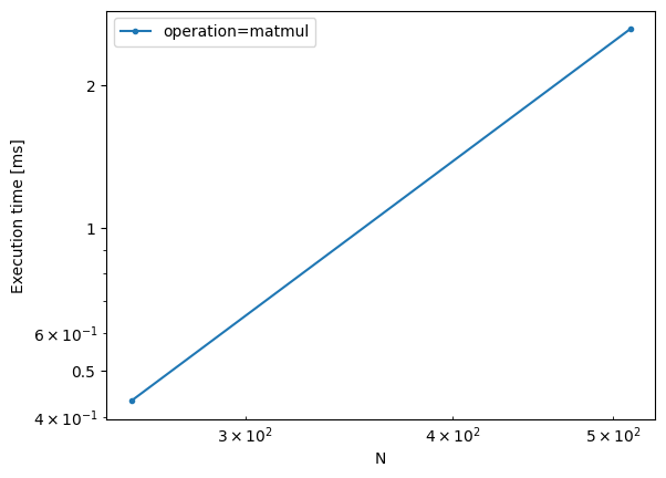
operation=matmul, N=256: 432.015 µs ± 1.16% (median of 7 runs, 500 loops each)
Setup code:
__bench_func = matmul
Benchmarked code:
__bench_func(a, b).block_until_ready()
operation=matmul, N=512: 2.621 ms ± 0.55% (median of 7 runs, 100 loops each)
print(bench)
┌───┬───────────┬─────┬─────────────┬──────────┬────────────┬────────────┬────────────┬────────────┐
│   ┆ operation ┆ N   ┆ median_exec ┆ ± (%)    ┆ first_exec ┆ compilatio ┆ generated_ ┆ temp_size  │
│   ┆           ┆     ┆ ution_time  ┆          ┆ ution_time ┆ n_time     ┆ code_size  ┆ (B)        │
│   ┆           ┆     ┆ (ms)        ┆          ┆ (ms)       ┆ (ms)       ┆ (B)        ┆            │
╞═══╪═══════════╪═════╪═════════════╪══════════╪════════════╪════════════╪════════════╪════════════╡
│ 0 ┆ matmul    ┆ 256 ┆ 0.432015    ┆ 1.15685  ┆ 11.35735   ┆ 0.235484   ┆ 0          ┆ 0          │
│ 1 ┆ matmul    ┆ 512 ┆ 2.620655    ┆ 0.548304 ┆ 11.549913  ┆ 0.255095   ┆ 0          ┆ 0          │
└───┴───────────┴─────┴─────────────┴──────────┴────────────┴────────────┴────────────┴────────────┘
Visualizing the Matrix Multiplication HLO
Display the HLO computational graph for the second run (N=128)
show(bench[1]['hlo'])

Plotting Results
bench.plot()